
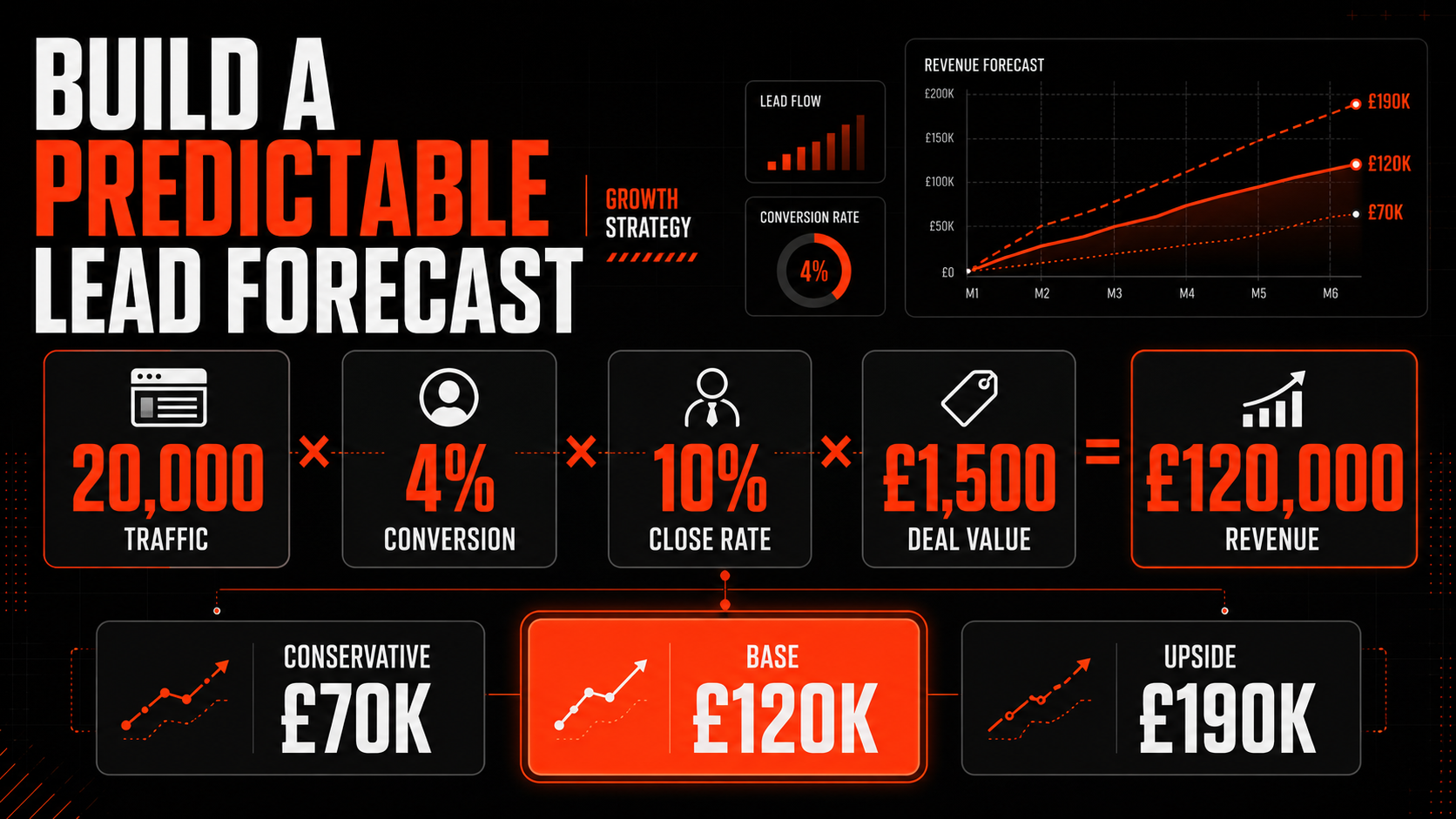
A predictable lead-generation forecast converts measurable funnel assumptions into expected leads, customers, revenue, contribution and cash timing. It should not begin with a revenue target and work backwards using optimistic conversion rates. It should combine historical traffic, visit-to-lead conversion, lead quality, sales close rate, deal-value mix and the delay between enquiry and sale.
The basic equation is:
Forecast revenue = Relevant traffic × Visit-to-lead rate × Lead-to-sale rate × Average deal value
A stronger commercial version is:
Forecast contribution after acquisition = Expected customers × Contribution per customer − Marketing and sales acquisition costs
These equations create a useful starting point, but predictability comes from the quality of the assumptions. A single blended rate can produce a mathematically correct yet commercially unrealistic forecast. The model should therefore be segmented, time-lagged, scenario-based and updated against mature customer cohorts.
The four variables in a lead-generation forecast
1. Relevant website traffic
Use the visits expected to reach lead-generating pages, not all site traffic. Blog readers, existing customers visiting support pages, job applicants and internal users may have little connection with the sales objective.
Forecast relevant traffic by source and landing-page group:
- Non-brand paid search.
- Brand search.
- Organic commercial pages.
- Organic informational content.
- Paid social.
- Email or returning prospects.
- Referral and partner traffic.
- Direct and unclassified traffic.
Each source can have a different conversion rate, customer value and sales cycle.
2. Visit-to-lead conversion rate
Visit-to-lead rate = Valid leads ÷ Relevant website visits × 100
Use valid, deduplicated leads. Remove spam, tests, job enquiries and contacts outside the company’s service criteria. If the forecast uses every form submission but sales reporting uses valid leads, the model will overstate opportunity.
3. Lead-to-sale conversion rate
Lead-to-sale rate = New customers ÷ Valid leads × 100
This rate combines lead quality with sales execution. For diagnosis, split it into stages:
Valid lead → Qualified lead → Sales opportunity → Proposal → Closed customer
4. Deal value
Use the expected mix of closed deals, not merely the historic arithmetic mean. A few unusually large contracts can inflate average deal value and make a normal month look like a forecast failure.
Where margin varies, forecast contribution value as well as revenue.
A complete worked example
Suppose the base assumptions for next month are:
- 20,000 relevant website visits.
- 4% visit-to-lead conversion.
- 12% lead-to-sale conversion.
- £1,500 average closed-deal value.
- 35% contribution margin before acquisition.
- £25,000 marketing and sales acquisition cost.
Expected leads:
20,000 × 4% = 800 leads
Expected customers:
800 × 12% = 96 customers
Expected revenue:
96 × £1,500 = £144,000
Expected contribution before acquisition:
£144,000 × 35% = £50,400
Expected contribution after acquisition:
£50,400 − £25,000 = £25,400
Expected fully loaded customer acquisition cost:
£25,000 ÷ 96 = £260.42
The forecast is not simply “£144,000 revenue”. It is 20,000 relevant visits producing 800 valid leads, 96 customers, £144,000 revenue and £25,400 contribution after acquisition—subject to the stated assumptions and sales-cycle timing.
Work backwards from a commercial target
A reverse model reveals what the revenue target requires.
Suppose the business wants £100,000 of new-customer revenue:
- Expected deal value: £2,000.
- Lead-to-sale rate: 10%.
- Visit-to-lead rate: 5%.
Required customers:
£100,000 ÷ £2,000 = 50 customers
Required valid leads:
50 ÷ 10% = 500 leads
Required relevant visits:
500 ÷ 5% = 10,000 visits
Now test feasibility:
- Can the available channels produce 10,000 relevant visits at the planned cost?
- Can the website maintain 5% conversion at that volume?
- Can sales process 500 leads without response time or quality deteriorating?
- Is there enough demand for 50 customers at the assumed deal value?
- Can operations deliver those customers profitably?
Reverse planning turns a board target into operational requirements. It also exposes a target that cannot be achieved within the available demand, capacity or budget.
Use historical conversion rates correctly
Your own first-party data is normally more useful than a generic benchmark. But historic rates must be comparable with the forecast period.
Do not blend together data from periods with materially different:
- Lead definitions.
- Traffic sources or campaign objectives.
- Website design and forms.
- Pricing and product mix.
- Sales team and capacity.
- Promotions.
- Geography.
- Seasonality and market demand.
- Attribution or tracking setup.
Use a hierarchy:
- Same segment and comparable recent period.
- Mature rolling three- or six-month rate.
- Same season last year, adjusted for known changes.
- Wider business average when segment volume is too small.
- External benchmark only as an explicitly labelled assumption.
For low-volume funnels, use a longer window. For rapidly changing businesses, weight recent performance more heavily while protecting the model from one unusual month.
Segment before you aggregate
Forecast each meaningful channel or customer segment separately, then add the results.
| Channel | Relevant visits | Visit-to-lead | Valid leads | Lead-to-sale | Customers | Deal value | Revenue |
|---|---|---|---|---|---|---|---|
| Organic search | 5,000 | 6% | 300 | 12% | 36 | £1,500 | £54,000 |
| Paid search | 8,000 | 4% | 320 | 10% | 32 | £2,000 | £64,000 |
| Paid social | 12,000 | 3% | 360 | 5% | 18 | £1,000 | £18,000 |
| Total | 25,000 | — | 980 | — | 86 | — | £136,000 |
Paid social creates the most leads, but the fewest customers and lowest revenue. A blended forecast using 25,000 visits, 3.92% visit-to-lead conversion, 8.78% lead-to-sale conversion and a single deal value arrives at the same total, but conceals why it is expected.
Segment by whichever dimensions materially alter the result:
- Channel and campaign.
- Product or service.
- Customer size.
- Geography.
- Landing page or offer.
- New and returning prospects.
- Salesperson or team.
- Deal-value band.
- Contract type.
- Sales-cycle length.
Forecast valid, qualified and sales-accepted leads
More forms do not necessarily create more pipeline. Include lead quality:
Expected qualified leads = Valid leads × Qualification rate
Expected opportunities = Qualified leads × Opportunity rate
Expected customers = Opportunities × Opportunity close rate
Suppose 800 valid leads produce:
- 50% qualified: 400.
- 60% opportunities: 240.
- 40% closed customers: 96.
This still equals 12% overall lead-to-sale conversion, but the stage model is more useful. If customers fall to 72, the business can see whether qualification, opportunity creation or closing caused the miss.
Google Analytics recommends lead-generation events including generate_lead, qualify_lead, working_lead and close_convert_lead. Its Lead acquisition report can use those stages to report new, qualified and converted leads. Google Analytics recommended events and Lead acquisition report
The CRM should remain the operational source for qualification, opportunity, forecast stage, owner and closed revenue.
Do not over-rely on average deal value
Suppose the previous period closed:
- 80 deals at £500.
- 20 deals at £5,000.
Total revenue is £140,000 and average deal value is £1,400. If the next month produces 100 deals but only five are in the larger band, using £1,400 will materially overstate revenue.
Forecast by deal band:
| Deal-value band | Expected deals | Expected average | Forecast revenue |
| Up to £1,000 | 60 | £600 | £36,000 |
| £1,001–£3,000 | 25 | £2,000 | £50,000 |
| Above £3,000 | 10 | £5,000 | £50,000 |
| Total | 95 | — | £136,000 |
Also consider median deal value. The median is often more stable where a small number of very large contracts distort the mean.
For subscription or retained services, distinguish:
- Contracted annual value.
- Recognised monthly revenue.
- Expected lifetime revenue.
- Cash collected.
Do not forecast all four as though they occur at the same time.
Forecast contribution, not revenue alone
A revenue forecast can be achieved while profit misses because the sales mix changes.
Calculate contribution per deal:
Contribution per deal = Deal revenue − Direct delivery cost − Product cost − Fulfilment − Payment fees − Commission − Expected refunds
Then:
Forecast contribution after acquisition = Sum of expected segment contribution − Marketing and sales acquisition costs
Example:
| Segment | Expected customers | Revenue per customer | Contribution per customer | Total contribution before acquisition |
| Entry service | 50 | £1,000 | £250 | £12,500 |
| Growth service | 25 | £3,000 | £1,200 | £30,000 |
| Enterprise | 5 | £15,000 | £6,000 | £30,000 |
| Total | 80 | — | — | £72,500 |
If acquisition cost is £35,000, forecast contribution after acquisition is £37,500.
The enterprise segment creates as much contribution as the 25 growth customers despite having far fewer sales. This is invisible in a lead-volume forecast.
Include sales-cycle timing
Demand generation, sales and recognised revenue occur at different times.
Measure the distribution of days between:
- First relevant visit and lead.
- Lead and qualification.
- Qualification and opportunity.
- Opportunity and proposal.
- Proposal and closed sale.
- Closed sale and invoice.
- Invoice and cash collection.
Use median and percentile ranges, not only the mean. A few very long deals can distort the average.
If 20% of a lead cohort normally closes in the same month, 50% in the following month and 30% two months later, allocate expected sales accordingly.
For 100 expected eventual customers from September leads:
- September: 20 sales.
- October: 50 sales.
- November: 30 sales.
This is more realistic than placing all 100 into September revenue.
Combine top-down demand with bottom-up pipeline
A strong forecast uses two views.
Top-down funnel forecast
Used for medium-term planning:
Traffic × Conversion rates × Customer value
It estimates future pipeline from expected demand.
Bottom-up opportunity forecast
Used for near-term sales:
Weighted pipeline = Sum of open opportunity value × Historic probability of closing in the period
Suppose the CRM contains:
| Stage | Open value | Historic period close rate | Weighted value |
| Qualified opportunity | £40,000 | 20% | £8,000 |
| Proposal | £60,000 | 50% | £30,000 |
| Negotiation | £30,000 | 75% | £22,500 |
| Total | £130,000 | — | £60,500 |
Use probabilities based on actual outcomes, not arbitrary labels such as “proposal = 50%”. Refine them by deal size, source, service, sales representative and opportunity age where volumes permit.
Reconcile the views:
- The pipeline view should explain the next few weeks or months.
- The funnel view should explain what later pipeline the marketing plan is expected to create.
- A large gap may reveal insufficient new demand, stale CRM opportunities or unrealistic stage probabilities.
Model sales-team capacity
A forecast can be mathematically achievable but operationally impossible.
Estimate:
- New leads per representative.
- Qualification time per lead.
- Contact attempts.
- Meetings and demos.
- Proposals.
- Active opportunities.
- Expected sales and onboarding handovers.
Suppose the plan creates 1,000 monthly leads. If one representative can properly manage 150 and there are four representatives, capacity is 600. The remaining 400 may wait, receive weaker follow-up or reduce conversion across the whole funnel.
Include a capacity-adjusted conversion assumption or resource plan. Do not assume historic close rate will survive a large volume increase without additional staffing, automation or qualification.
Account for marketing capacity and diminishing returns
Traffic does not normally scale in a straight line.
Paid media may reach weaker queries and audiences as budgets rise. SEO and content may need months to build traffic. Referral volume may be efficient but constrained. Paid social may depend on creative production.
For each channel, model:
- Current traffic and cost.
- Available demand or audience.
- Cost of the next traffic increment.
- Expected conversion at higher volume.
- Implementation or creative lead time.
- Saturation risk.
Do not forecast a 20% traffic increase by multiplying spend by 1.2 unless historical marginal performance supports it.
Build conservative, base and upside scenarios
A single number creates false precision.
| Scenario | Visits | Visit-to-lead | Leads | Lead-to-sale | Customers | Deal value | Revenue |
| Conservative | 18,000 | 3.5% | 630 | 8% | 50 | £1,400 | £70,000 |
| Base | 20,000 | 4.0% | 800 | 10% | 80 | £1,500 | £120,000 |
| Upside | 22,000 | 4.5% | 990 | 12% | 119 | £1,600 | £190,400 |
The upside case is dramatically higher because the variables multiply. It should represent a plausible favourable outcome, not a target disguised as a forecast.
Use:
- Conservative case for cash and minimum capacity planning.
- Base case for normal operating plans.
- Upside case for contingency stock, staffing and delivery capacity.
Add contribution and cash timing to each scenario.
Run sensitivity analysis
Sensitivity analysis shows which assumption matters most.
Using the 20,000-visit base:
| Change | Leads | Customers | Revenue at £1,500 |
| Baseline: 4% lead rate, 10% close | 800 | 80 | £120,000 |
| Lead rate improves to 5% | 1,000 | 100 | £150,000 |
| Close rate improves to 12% | 800 | 96 | £144,000 |
| Both improvements | 1,000 | 120 | £180,000 |
| Deal value rises to £1,700 only | 800 | 80 | £136,000 |
This helps prioritise investment. If a realistic sales-process improvement creates more contribution than buying additional traffic, the budget should follow the constraint rather than a departmental preference.
Forecast by salesperson carefully
Sales conversion and deal value can vary by representative.
Track:
- Leads assigned and accepted.
- Contact and qualification rates.
- Opportunities, proposals and wins.
- Lead-to-sale rate.
- Average and median deal value.
- Sales-cycle length.
- Contribution sold.
Control for source, territory, customer type, service and deal complexity before using individual rates. A representative working enterprise opportunities may close fewer deals with a longer cycle but create greater contribution.
Use individual forecasting only where volume is sufficient; otherwise use team or segment rates to avoid overreacting to random variation.
Measure assisted journeys without double-counting
A lead may discover the business through paid social, return through organic search and submit through a brand advert. Assigning the full forecasted customer to every channel would double-count revenue.
Use one primary planning allocation and an assisted-journey view alongside it. Google Analytics’ attribution-paths report can show channels that initiate, assist and close key events, along with touchpoints and days to conversion. Google Analytics attribution paths
Attribution helps explain paths, but it does not prove incrementality. Keep total forecast customers reconciled with the CRM and finance forecast regardless of how credit is distributed.
Track forecast accuracy at every stage
Do not assess only final revenue.
For a positive actual value, a simple absolute accuracy measure is:
Forecast accuracy = 1 − Absolute value of (Actual − Forecast) ÷ Actual
If this produces a negative percentage after a very large miss, report the absolute percentage error instead; the stage variance is more important than forcing a friendly score.
Track forecast versus actual for:
- Relevant visits.
- Cost per visit.
- Valid and qualified leads.
- Visit-to-lead conversion.
- Opportunities.
- Lead-to-sale conversion.
- Sales timing.
- Deal-value mix.
- Revenue.
- Contribution.
- Acquisition cost and payback.
Use a variance bridge:
| Forecast miss | Likely assumption to review |
| Traffic below plan | Channel demand, budget, delivery or seasonality |
| Leads below plan | Landing-page conversion, offer or traffic quality |
| Qualified leads below plan | Targeting, message or qualification assumptions |
| Opportunities below plan | Sales acceptance, discovery or customer fit |
| Sales below plan | Close rate, capacity, competition or cycle delay |
| Revenue below plan with sales on target | Deal-value mix or discounting |
| Contribution below plan with revenue on target | Margin, delivery cost or sales mix |
| Cash below plan with sales on target | Invoice timing, terms or collection |
Update the assumption that failed rather than changing the final revenue number without explanation.
Set a practical reporting cadence
Weekly
- Traffic and media delivery.
- Lead volume and validity.
- Response time.
- Qualification and opportunity creation.
- Pipeline movement and slippage.
- Capacity constraints.
Monthly
- Mature conversion by cohort.
- Closed customers and deal-value mix.
- Revenue, contribution and CAC.
- Scenario variance.
- Revised rolling forecast.
Quarterly
- Channel and customer cohort economics.
- Sales-cycle distribution.
- Retention and lifetime contribution.
- Forecast bias and accuracy.
- Budget, staffing and capacity changes.
Avoid rewriting historic forecasts. Preserve the original forecast, the date it was made, the assumptions and every later revision so the business can learn where bias enters the model.
A practical forecasting template
For each segment, include:
| Input or output | Example |
| Relevant traffic | 5,000 |
| Traffic cost | £10,000 |
| Visit-to-valid-lead rate | 5% |
| Valid leads | 250 |
| Qualification rate | 50% |
| Qualified leads | 125 |
| Opportunity rate | 60% |
| Opportunities | 75 |
| Opportunity close rate | 33.3% |
| Customers | 25 |
| Average deal value | £4,000 |
| Revenue | £100,000 |
| Contribution per customer | £1,800 |
| Contribution before acquisition | £45,000 |
| Marketing and sales acquisition cost | £20,000 |
| Contribution after acquisition | £25,000 |
| Fully loaded CAC | £800 |
| Median sales cycle | 45 days |
Add conservative, base and upside values for the important assumptions and state the source period for every rate.
The practical answer
Build a predictable lead-generation forecast using:
Expected revenue = Relevant traffic × Visit-to-lead rate × Lead-to-sale rate × Expected deal value
For a more commercially useful result:
Expected contribution after acquisition = Sum of expected customers by segment × Contribution value per customer − Marketing and sales acquisition costs
Segment the model by channel, customer type, product or service and deal band. Use mature historic conversion rates, account for lead quality and sales capacity, and distribute sales according to the actual sales-cycle lag.
Combine a top-down funnel forecast with a bottom-up weighted pipeline. Use conservative, base and upside scenarios, then compare each assumption with actual results so the model becomes more accurate over time.
Predictability does not mean the result will be exact. It means the business understands the range of likely outcomes, the assumptions driving them, the time at which revenue should arrive and the action required when one stage moves off plan.
Book a Strategy Call
If your lead and revenue targets are based on historic growth percentages rather than validated funnel economics, Clubbish can build a forecast connecting channel demand, website conversion, sales performance, customer value, contribution and cash timing. We will identify the assumptions limiting predictability and create a practical model for budget, capacity and growth decisions.